Figure 1From “What is Little's law?”
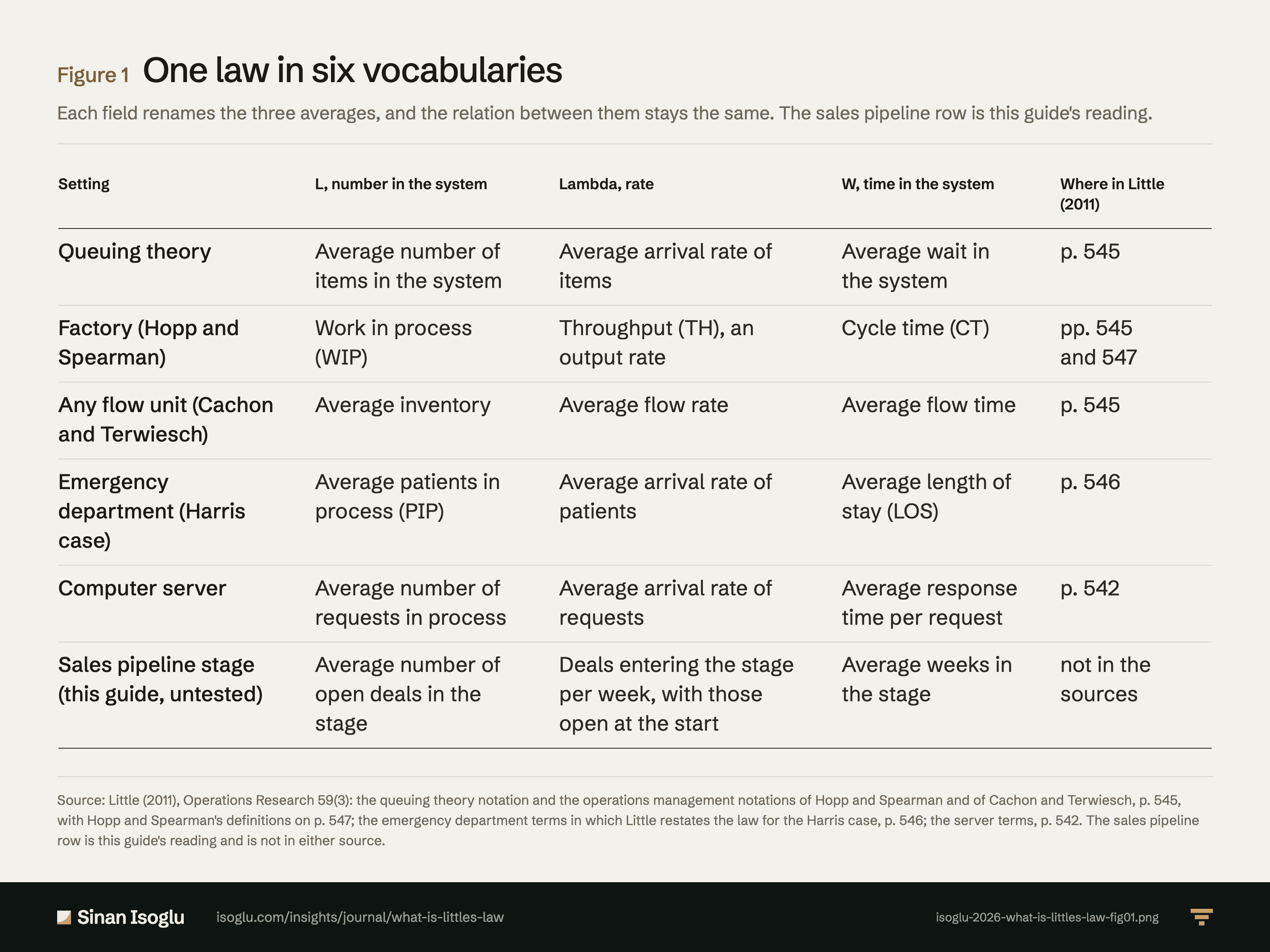
One law in six vocabularies
Each field renames the three averages, and the relation between them stays the same. The sales pipeline row is this guide's reading.
Figure 1One law in six vocabularies
| Setting | L, number in the system | Lambda, rate | W, time in the system | Where in Little (2011) |
|---|---|---|---|---|
| Queuing theory | Average number of items in the system | Average arrival rate of items | Average wait in the system | p. 545 |
| Factory (Hopp and Spearman) | Work in process (WIP) | Throughput (TH), an output rate | Cycle time (CT) | pp. 545 and 547 |
| Any flow unit (Cachon and Terwiesch) | Average inventory | Average flow rate | Average flow time | p. 545 |
| Emergency department (Harris case) | Average patients in process (PIP) | Average arrival rate of patients | Average length of stay (LOS) | p. 546 |
| Computer server | Average number of requests in process | Average arrival rate of requests | Average response time per request | p. 542 |
| Sales pipeline stage (this guide, untested) | Average number of open deals in the stage | Deals entering the stage per week, with those open at the start | Average weeks in the stage | not in the sources |
Swipe or scroll horizontally if the table is wider than your screen.
Source: Little (2011), Operations Research 59(3): the queuing theory notation and the operations management notations of Hopp and Spearman and of Cachon and Terwiesch, p. 545, with Hopp and Spearman's definitions on p. 547; the emergency department terms in which Little restates the law for the Harris case, p. 546; the server terms, p. 542. The sales pipeline row is this guide's reading and is not in either source.
Source and evidence
Each line names a claim related to this exhibit, its source, and how it was checked.
- A LIT11-C9 The law in field vocabularies: queuing theory L, λ, W; Hopp and Spearman TH = WIP/CT with throughput, work in process and cycle time, which Little quotes as the average output of a production process per unit time, the inventory between the start and end points of a routing, and the time from release of a job at the beginning of the routing to its end; Cachon and Terwiesch average inventory, flow rate and flow time; emergency department patients in process, arrival rate and length of stay, the terms in which Little himself restates the law for the Harris case, borrowing operations management terminology for patients in process; the held source does not say which terms Harris used (revised after G5 F6); server requests in process, arrival rate of requests and response time; operations management states the law with the output rate rather than the arrival rate, and in many settings the arrival process is in effect endogenous; operations management applications draw their vocabulary from the client setting (G5 N6) (pp. 542, 545 to 547): "average number of requests in process"; "average response time per request"; "throughput (items/unit time)"; "work in process (items)"; "cycle time (time units/item)"; "Average Inventory = Average Flow Rate"; "Average Flow Time"; "rate or flow rate for the system, rather than the arrival rate"; "In effect, the arrival process is endogenous"; "LOS fits easily into Little's Law"; "average patients in process"; "given the acronym PIP. So, rewriting Little"; "the average output of a production process"; "the inventory between the start and end points"; "time from release of a job at the beginning of the routing"; "One of the characteristics of OM applications of"; "Law is to draw the vocabulary for the application from"; "jargon of the client setting"Little (2011) · Little. (2011)
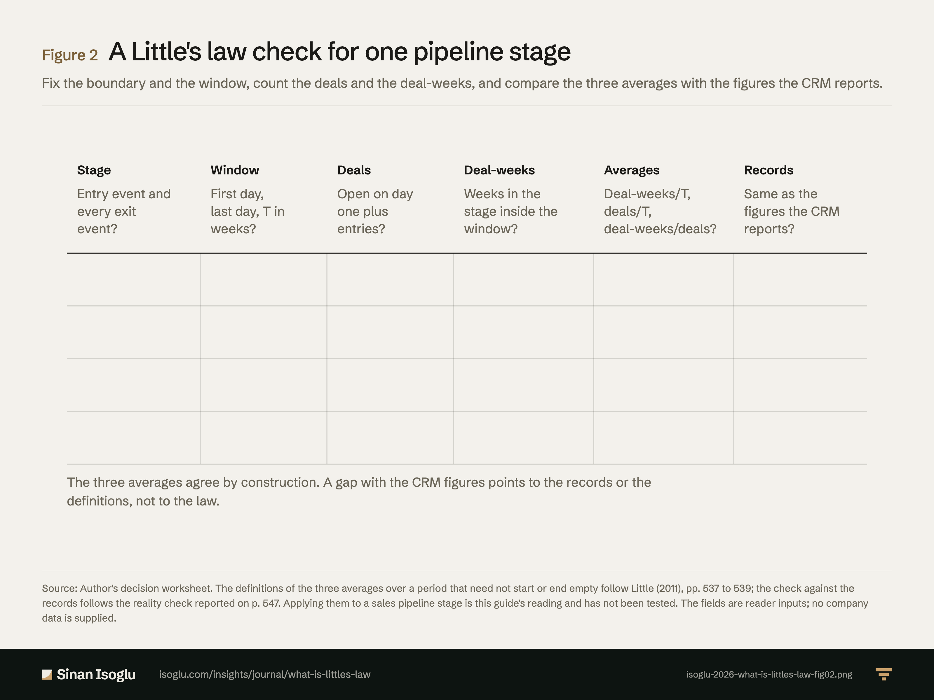
- B LLAW-OWN-C3 A pipeline stage read with the finite-period law (author's example, invented numbers, untested): the system is one stage bounded by its entry event and every exit (advanced, moved back to an earlier stage, won, lost, disqualified), a deal moved back into the stage counts as a new arrival; over 13 weeks, 120 deals open on day one and 270 entries give 390 deals, 1,560 deal-weeks give L = 120, λ = 30 per week, W = 4 weeks (day-one count revised after G5 N7, exits after N8); two of the three give the third; without dates, averaged weekly counts approximate L, and divided by λ, which includes the deals open on day one, they give W, while dividing by the entries alone gives a different number (5.8 weeks on these numbers), not the finite-period W (G5 F2); computed from one set of dates the three agree by construction; a gap with the CRM's own figures points to the records or the definitions (rewritten entry dates, a CRM time in stage taken only from deals that left), and lost deals left open show as a slower stage, not as a gap (revised after G5 F1); at a constant λ of 30 deals a week, a rise from 120 to 150 open deals means W rose from 4 to 5 weeks; the law cannot say why, nor give win rates, values or forecasts; Figure 1's last row and the Figure 2 worksheet.Author worksheet grounded in LIT61-C4, LIT11-C6, LIT11-C7 and LIT11-C10; untested
Grades: A, verified against the printed page of the primary source · B, primary source, text layer only · C, authoritative secondary · D, reported.
From the essay
Revenue operations & AI
What is Little's law?
Little's law, L = λW, ties three averages: items in a system, the rate they arrive and the time each spends inside. It measures and does not explain.
Read the essayThis exhibit belongs to an essay: the numbers live here, the argument lives there.
Cite or embed
Contact
Bring the question you're working on.
Research, a guest lecture, or a commercial question.