Abbildung 1Aus „Was ist Zeitreihenprognose?“
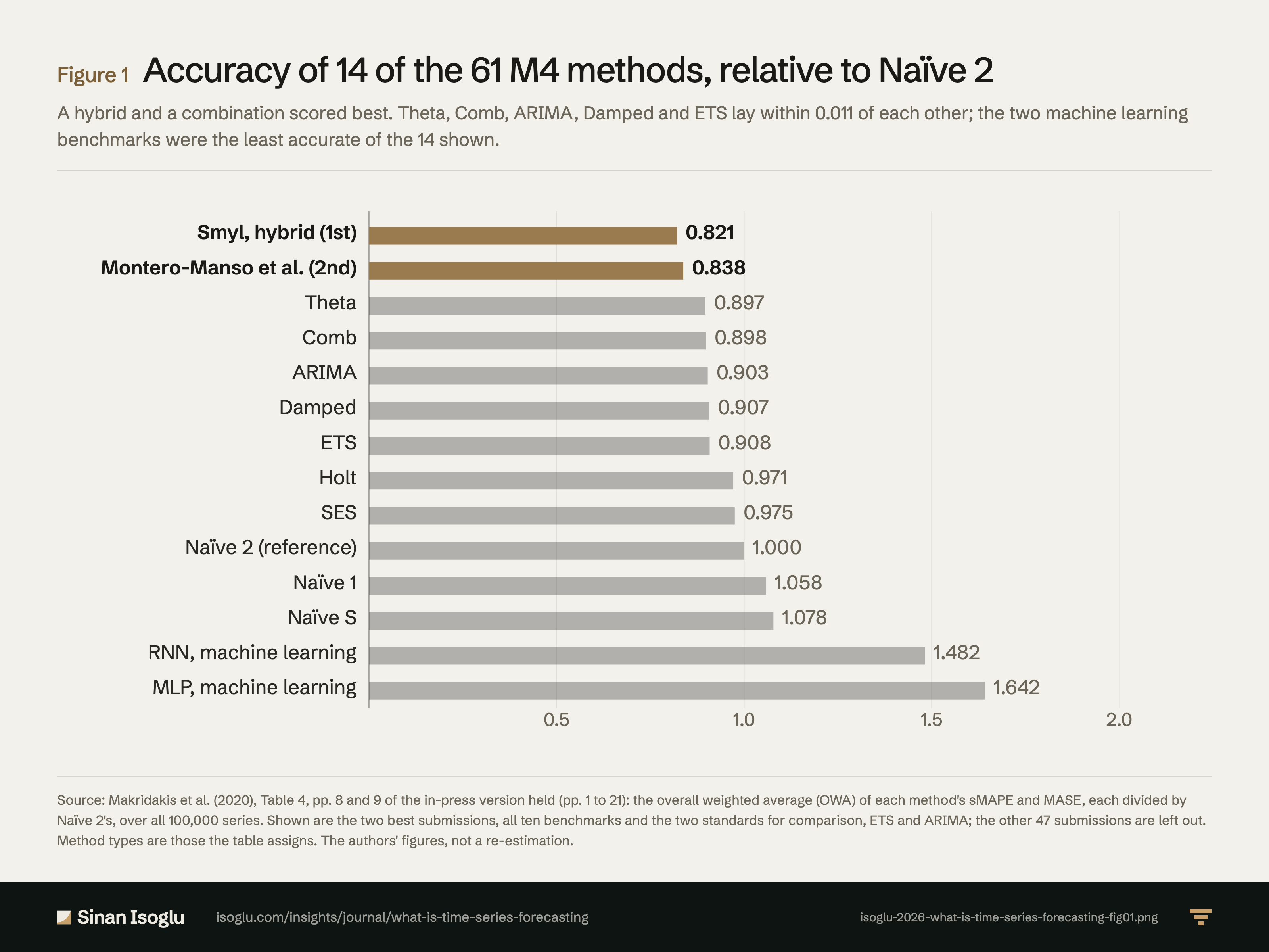
Genauigkeit von 14 der 61 M4-Verfahren, relativ zu Naïve 2
Ein hybrides Verfahren und eine Kombination lagen vorn. Theta, Comb, ARIMA, Damped und ETS lagen höchstens 0,011 auseinander; die beiden Benchmarks des maschinellen Lernens waren von den 14 gezeigten Verfahren am ungenauesten.
Abbildung 1Genauigkeit von 14 der 61 M4-Verfahren, relativ zu Naïve 2
Quelle: Makridakis et al. (2020), Tabelle 4, S. 8 und 9 der vorliegenden Vorabfassung (Article in Press, S. 1 bis 21): das OWA (Overall Weighted Average) aus sMAPE und MASE jedes Verfahrens, jeweils geteilt durch den Wert von Naïve 2, über alle 100.000 Reihen. Gezeigt sind die beiden besten Einreichungen, alle zehn Benchmarks und die beiden Vergleichsstandards ETS und ARIMA; die übrigen 47 Einreichungen sind weggelassen. Die Verfahrenstypen sind die, die die Tabelle angibt. Werte der Autoren, keine Neuberechnung.
Quelle und Evidenz
Jede Zeile nennt eine Aussage zu dieser Abbildung, ihre Quelle und die Art ihrer Prüfung.
- A MSA20-C4 Combining: all top-performing methods were combinations of mostly statistical methods and only one pure statistical method was in the top ten, while all of the ten least accurate were pure statistical or pure ML (six statistical, four ML in Table 4); the two least accurate of all 61, Dudek (OWA 2.561, rank 60) and Sirotin (4.387, rank 61), are statistical submissions that Figure 1 leaves out (Table 4, p. 9, read again from the page image after G5 F1); Table 4 (pp. 8 and 9, read from page images) classes the winner as a hybrid and ranks two to six as combinations, and gives OWA Theta 0.897, Comb 0.898, ARIMA 0.903, Damped 0.907, ETS 0.908, Holt 0.971, SES 0.975, Naïve 2 1.000, Naïve 1 1.058, Naïve S 1.078 (the same values for the seven methods of Table 6, p. 11); Theta, Comb, ARIMA, Damped and ETS are the five best of the twelve benchmarks and standards and lie within 0.011, and Table 4 classes Comb as a combination, not as a statistical method, so the page calls the five the best benchmarks and standards (G5 F1); Comb more accurate than each of its three components; combining does not guarantee beating single models, and Theta, a single method and the most accurate of M3, beat Comb, ARIMA and ETS; Damped, Comb and ARIMA very similar, with hardly any statistically significant differences by Fig. 1, a multiple comparisons with the best test on sMAPE ranks; ARIMA's edge over ETS small and not significant (pp. 7 to 9, 11, 12, 15, 16 and 18 of the in-press version): "all of the top-performing methods, in terms of both PFs and PIs, were combinations of mostly statistical methods"; "there was only one pure statistical method among the first ten most-accurate ones"; "while all of the ten least-accurate methods were either pure statistical or pure ML"; "The poor performances of pure statistical and ML methods"; "In this table, Comb provides more accurate PFs than the three individual methods being combined."; "combining does not guarantee that their forecasts will outperform single models"; "the most accurate method of the M3 Competition"; "Theta provides more accurate PFs than Comb, ARIMA and ETS, despite utilizing a simple approach to forecasting"; "The numerical accuracies of Damped, Comb and ARIMA are very similar in M4"; "Fig. 1 indicates that hardly any statistically significant differences among the methods can be found"; "multiple comparisons with the best (sMAPE used for ranking the methods)"; "Even though the improvement is small, and not statistically significant according to Fig. 1"Makridakis, Spiliotis & Assimakopoulos (2020) · Makridakis, Spiliotis & Assimakopoulos. (2020)
- A MSA20-C5 The winner (Smyl, OWA 0.821) mixes exponential smoothing formulas with a recurrent neural network, its parameters fitted together with the network weights; its improvement over Comb is close to 10% (Table 4: 9.4% on sMAPE, 8.6% on OWA); second (Montero-Manso et al., 0.838) is a combination of seven statistical methods and one machine learning method whose weights a machine learning algorithm set for each series; five machine learning methods were submitted (four pure, one combination), all less accurate than Comb and only one more accurate than Naïve 2; the RNN and MLP benchmarks scored 1.482 and 1.642 (Table 4); the authors' possible reasons are a conjecture (limited cross-learning, short series, over-fitting, non-stationarity), and they say the paucity of entries limits generalization (pp. 4, 8, 9, 11, 12 and 15 of the in-press version): "which mixes ES formulas with a recurrent neural network (RNN) forecasting engine"; "are fitted concurrently with the RNN weights by the same gradient descent method"; "The improvement of this method over that of Comb was close to an impressive 10%"; "The second most accurate method in terms of PFs was a combination of seven statistical methods and a ML one"; "being calculated by a ML algorithm that was trained to minimize the forecasting errors through holdout tests for each individual series"; "A total of five ML methods (four pure and one combination) were submitted in M4."; "All of them were less accurate than the Comb benchmark in terms of PFs, and only one was more accurate than the Naïve 2 method."; "could be the limited usage of cross-learning"; "the limited usage of cross-learning, i.e., using information from multiple series to predict individual ones, together with the limited sample sizes of the individual series, the effect of over-fitting and the non-stationarity of the data"; "given the paucity of entries in the ML category, more information might still be needed to make it safe to generalize this finding"Makridakis, Spiliotis & Assimakopoulos (2020) · Makridakis, Spiliotis & Assimakopoulos. (2020)
Prüfgrade: A, gegen die gedruckte Seite der Primärquelle geprüft · B, Primärquelle, nur Textebene · C, belastbare Sekundärquelle · D, berichtet.
Aus dem Beitrag
Revenue Operations & KI
Was ist Zeitreihenprognose?
Zeitreihenprognose schreibt Reihen aus ihrer Vergangenheit fort. Im M4-Wettbewerb führten ein Hybrid und Kombinationen; reine Verfahren fielen zurück.
Den Beitrag lesenDiese Abbildung gehört zu einem Essay: Die Zahlen stehen hier, das Argument dort.
Zitieren oder einbetten
Verwandte Abbildungen
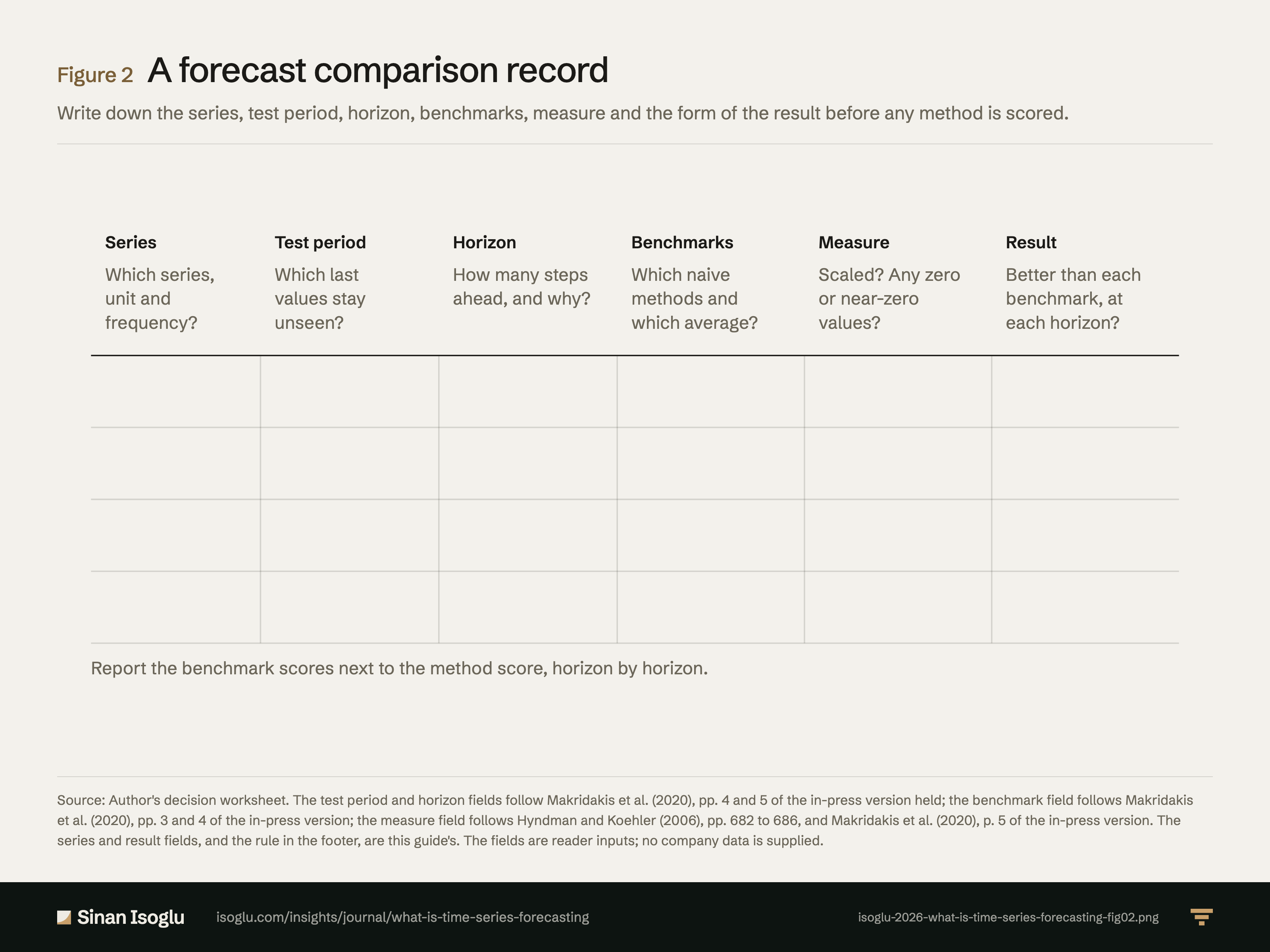
Abbildung 2Grafik
Ein Blatt für einen Prognosevergleich
Was ist Zeitreihenprognose?
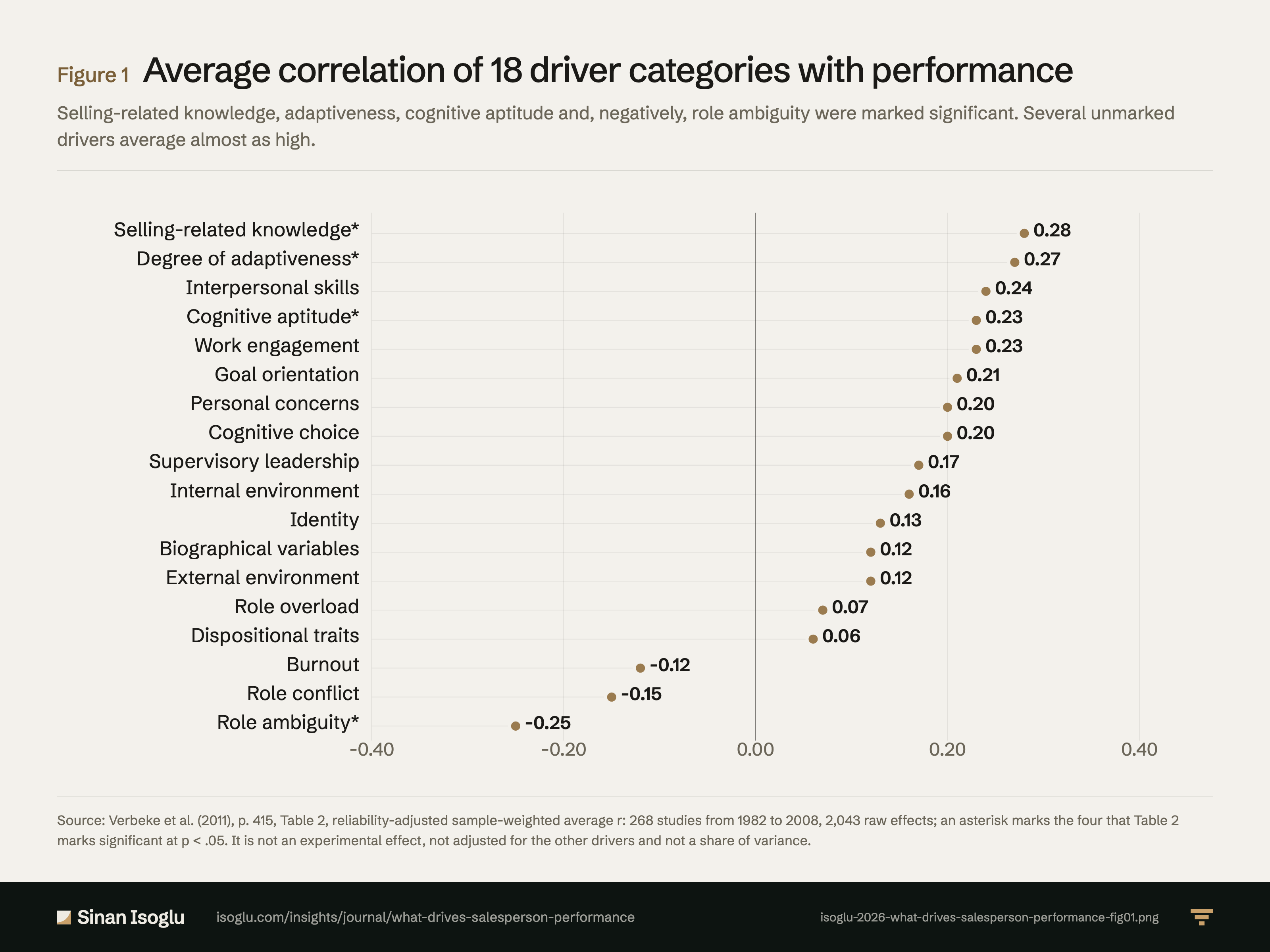
Abbildung 1Grafik
Mittlere Korrelation von 18 Kategorien mit der Verkaufsleistung
Was bestimmt die Leistung im Verkauf?
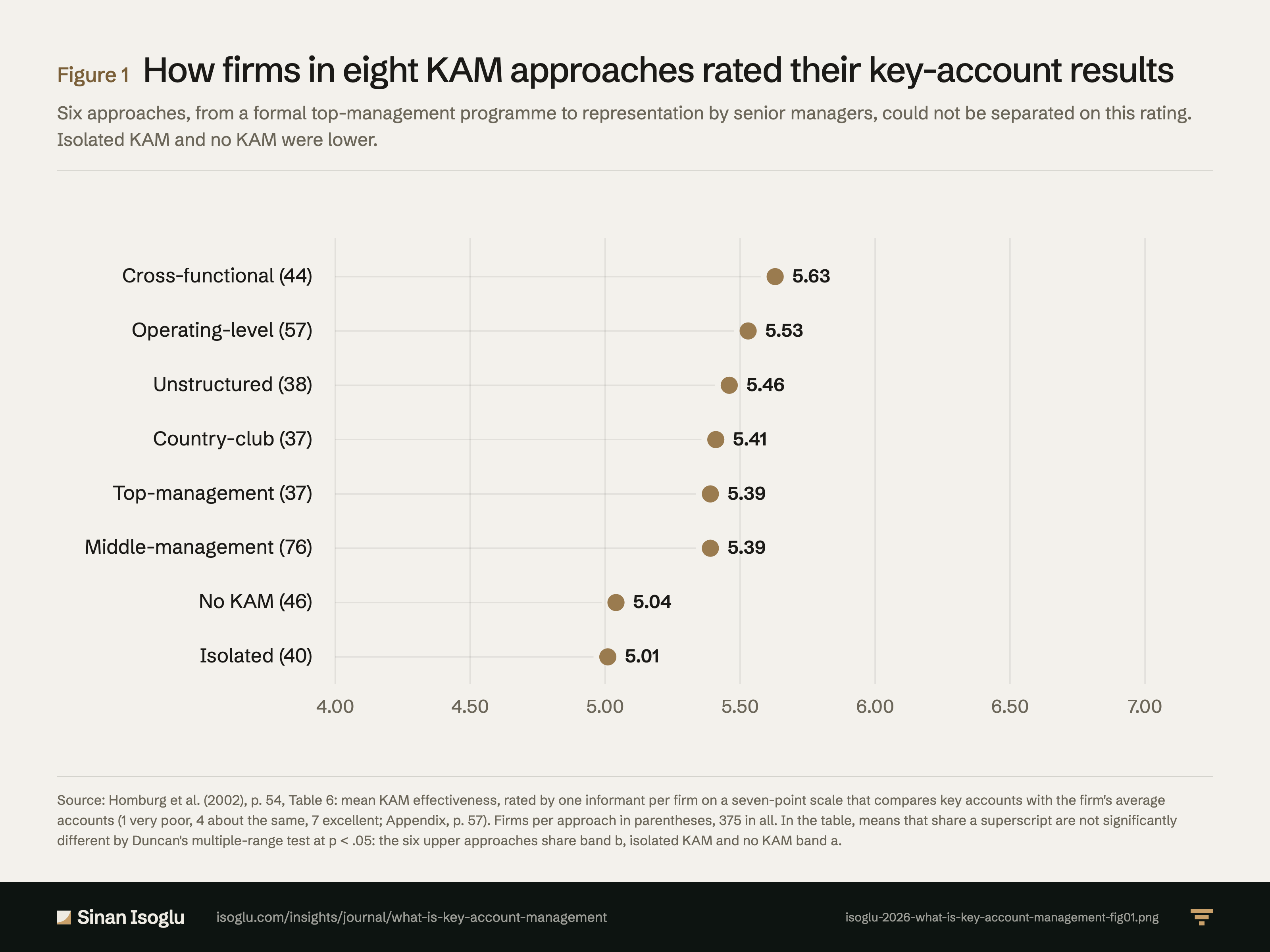
Abbildung 1Grafik
Ergebnisse mit Key Accounts, bewertet nach acht KAM-Ansätzen
Was ist Key Account Management?
Kontakt
Schicken Sie die Frage, an der Sie arbeiten.
Forschung, ein Gastvortrag oder eine Frage aus der Praxis.